Generating a periodic system for FHI-aims (sub system)

Objective: Turn a sub system of the MD system into a geometry file suitable for FHI-aims to be simulated with periodic boundary conditions.

Specifically, we want to select a box around the solute that extends 5 Å in all directions and only include the solvent molecules in this buffer zone together with the solute.

Danger

Unlike when we were exporting the full MD system, which was simulated under periodic boundary conditions, here we are cutting out a orthorhombic sub-system that is not truly periodic. We are assuming that the solvent is sufficiently homogeneous so that the newly introduced periodic boundaries do not introduce substantial artifacts such as clashes due to wrapped atoms or incorrect local coordination geometry. In practice, such a reduced system will likely have clashes and require additional work to be suitable for running in FHI-aims.

Despite these potential problems with intermolecular interactions, the protocol described here will ensure that intramolecular bonds are correctly wrapped around the new unit cell. The resulting system should be carefully examined and if necessary, additional steps such as energy minimization with the classical force field under the new periodic boundary conditions are necessary. Below we sketch out an example protocol for how to use GROMACS to do such an energy minimization to remove clashes.

Warning

This tutorial assumes that the MD trajectory was simulated inside a orthorhombic unit cell (i.e., all angles 90°); the simple approach shown here will not work correctly for non-orthorhombic unit cells. (Although MDAnalysis works with all unit cells, the simple cutting and rewrapping step used here requires orthorhombic unit cells.)

Protocol

The following commands can be used interactively in the python or ipython interpreter or a Jupyter notebook. Alternatively, combine them in a script extract_reduced_pbc.py and run the script with python extract_reduced_pbc.py.

Set-up, Centering, Trajectory frame selection

Import NumPy, MDAnalysis and the MDAnalysis transformations module:

import numpy as np
import MDAnalysis as mda
from MDAnalysis import transformations

Load the topology (TPR) and trajectory (TRR) of the classical MD simulation into the universe u:

u = mda.Universe("./files/MD/NPT/md.tpr", "./files/MD/NPT/md.trr")

Classical MD system on the last frame of the trajectory. Water molecules (AtomGroup `water`) are shown in CPK and the solute (AtomGroup `solute`) in VDW representation; the unit cell is shown as a blue cubic box. (Note that PBC artifacts have been fixed in this image to show the selections more clearly. See the next section for what this system *actually* looks like.)

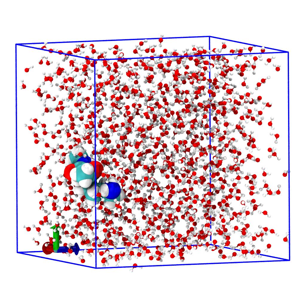
The following steps are the same as in the Set-up step for the full MD system (and following steps) so we will only summarize them here.

1. Change atom names to elements.
2. Create AtomGroup instances for the water molecules (water) and the solute by using selection by residue name and checking that we selected everything.
3. Center the system.
4. Move to the last frame of trajectory.

u.atoms.names = u.atoms.elements

water = u.atoms.select_atoms("resname SOL")
solute = u.atoms.select_atoms("resname ACE LYSN NME")
assert u.atoms == solute + water

workflow = [transformations.unwrap(u.atoms),
            transformations.center_in_box(solute, center='geometry'),
            transformations.wrap(water, compound='atoms')]
u.trajectory.add_transformations(*workflow)

u.trajectory[-1]

System after centering on the solute (lysine in VDW representation) and wrapping all atoms of water molecules back into the box of the periodic unitcell. Water molecules are broken across the periodic boundary, which is the correct behavior.

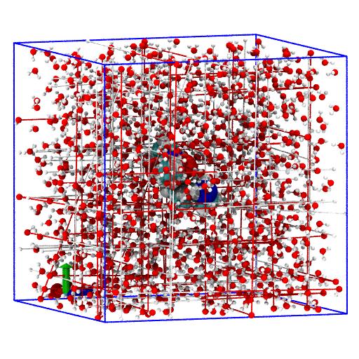
Find new reduced unit cell

Solute bounding box

We first find the bounding box of the solute (the orthorhombic cell with axes parallel to the coordinate system that exactly fits the solute in its current orientation) with the AtomGroup.bbox() method:

bbox = solute.bbox()

The variable bbox = [[xmin, ymin, zmin], [xmax, ymax, zmax]] contains the lower and upper corner of the enclosing bounding box.

For our information we compute the lengths A, B, C of the bounding box and compare them to the current dimensions of the unit cell.

A, B, C = bbox[1] - bbox[0]
print("unit cell:   a={uc[0]:7.4f} Å  b={uc[1]:7.4f} Å  c={uc[2]:7.4f} Å  ⍺={uc[3]}° β={uc[4]}° ɣ={uc[5]}° ".format(uc=u.dimensions))
print(f"solute bbox: A={A:7.4f} Å  B={B:7.4f} Å  C={C:7.4f} Å")

Warning

If the angles of the unit cell are not all equal to 90° then stop here. This protocol will only work for orthorhombic unit cells.

For the example files the output is

unit cell:   a=31.0358 Å  b=31.0358 Å  c=31.0358 Å  ⍺=90.0° β=90.0° ɣ=90.0°
solute bbox: A= 7.8396 Å  B= 7.3349 Å  C= 7.0937 Å

New orthorhombic unit cell

We add a distance of

delta = 5

in all directions

rmin = bbox[0] - delta
rmax = bbox[1] + delta

(extend the lower corner of the bounding box by -delta and the upper corner by +delta). rmin now contains the coordinates of the lower left front corner of the new unit cell (centered on the solute) and rmax are the coordinates of the upper right back corner.

Tip

Change delta to fit your own requirements. Visually check the reduced system once you write it out after the last step. Make sure that there are no clashes and that there is a sufficient solvation shell around the solute; "sufficient" is determined by the scientific question that you want to answer.

Select water in new unit cell

We select complete molecules with the byres selection keyword inside the extended box around the solute and use a boolean and selection with the prop selection keyword to find all water atoms that have their coordinates within the limits of our delta-expanded bounding box:

\[\begin{align} x_\text{min} - \delta < &x < x_\text{max} + \delta\\ y_\text{min} - \delta < &y < y_\text{max} + \delta\\ z_\text{min} - \delta < &z < x_\text{max} + \delta\ \end{align}\]

water_box = water.select_atoms(f"byres prop x > {rmin[0]} and prop x < {rmax[0]} and "
                               f"prop y > {rmin[1]} and prop y < {rmax[1]} and "
                               f"prop z > {rmin[2]} and prop z < {rmax[2]}")

Create combined system with new unit cell

Combine solute and the reduced water system into our reduced sub-system:

smaller_system = solute + water_box

Reduced system of the solute (lysine in VDW representation) and all water molecules inside the new unit cell, formed by expanding the bounding box of the solute by 5 Å. The original larger unit cell is shown in blue.

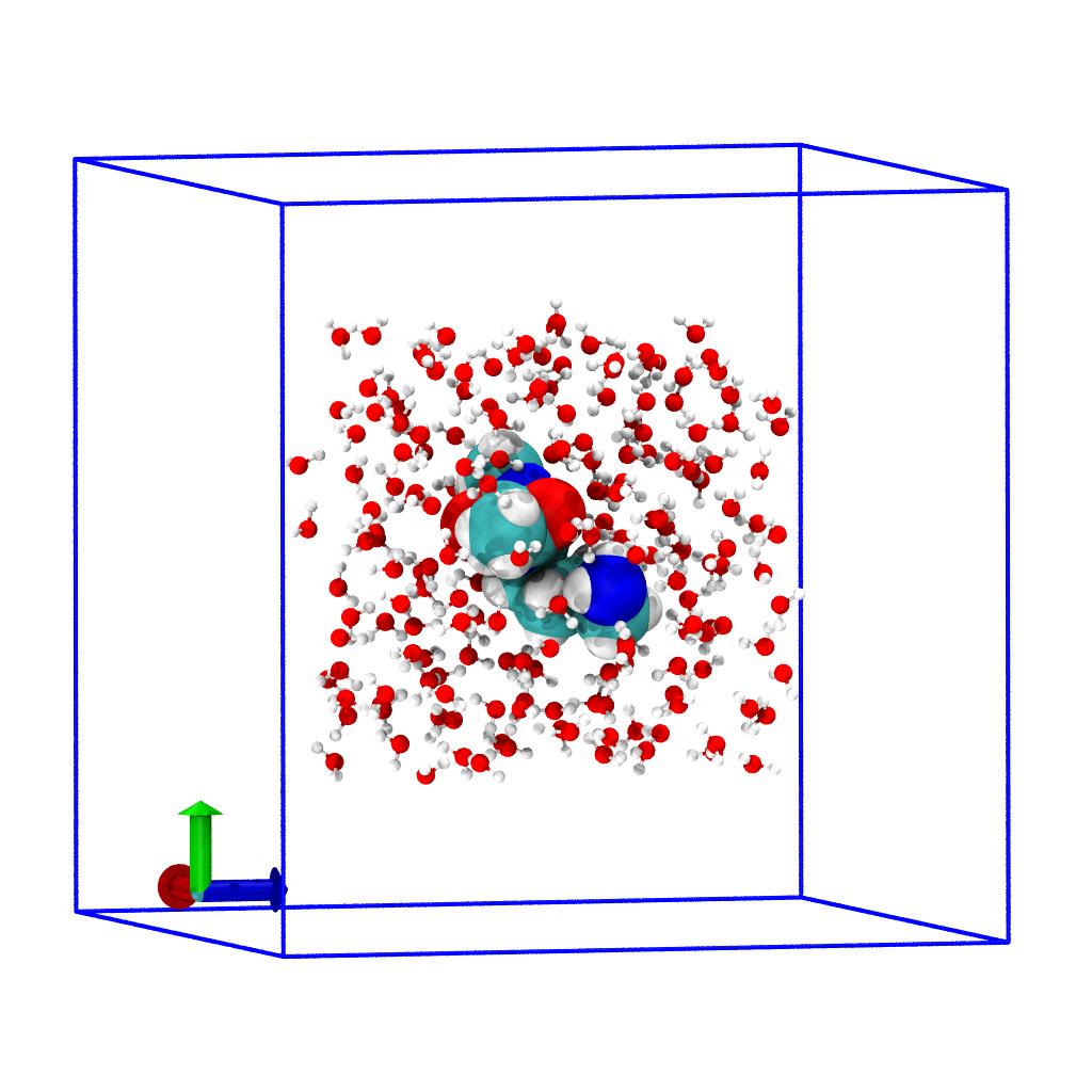
The dimensions of the new orthorhombic unit cell are [A, B, C, 90, 90, 90]:

newbox = np.concatenate([rmax - rmin, [90, 90, 90]])

In MDAnalysis, unit cells are always oriented in such a way that the unit cell vectors originate in \((0, 0, 0)\), that the first box vector is parallel to the Cartesian \(x\) axis \((1, 0, 0)^T\), the plane spanned by the first and second unit cell vector lies in the Cartesian \(xy\) plane, and the third vector should be oriented into the positive-\(z\) half-space to form a right-handed coordinate system.

In the next steps we will apply coordinate transformations to make our new reduced system conform to the unit cell requirements of MDAnalysis.

Note

All coordinate transformations that follow are temporary in that they change the current system coordinates but they will all be overwritten and forgotten when the trajectory is moved to another frame (e.g. u.trajectory[2]); we will write out the currently altered coordinates to save them (Alternatively, we could use in-memory trajectories to make changes permanent but that is a more advanced topic.)

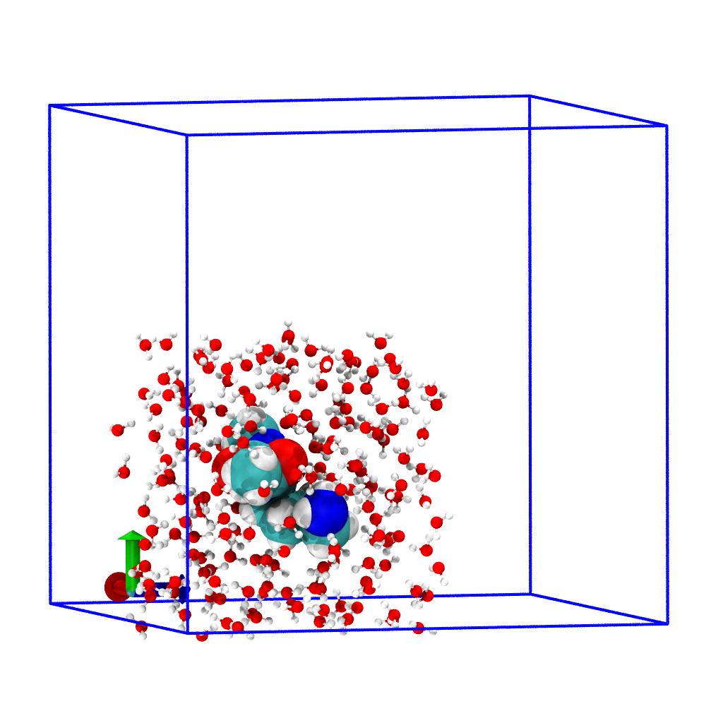
The new unit cell will have lower left corner (0,0,0) so lets shift all coordinates of the system accordingly; this will ensure that our small system (which is still part of the full system u.atoms) will be positioned so that its lower left front corner will be located at the origin:

u.atoms.translate(-rmin)

The reduced system was translated so that its lower left front corner coincides with the origin of the coordinate system. The original larger unit cell is shown in blue.

Set new unit cell dimensions and wrap atoms

Set the new unit cell dimensions

smaller_system.dimensions = newbox

so that the correct unit cell is written to output.

Note on how .dimensions is really changed globally.

This command actually sets dimensions for the whole Universe because .dimensions is really a property of the trajectory and is thus shared between all AtomGroups of the same Universe. Like the changing of positions, this change is only temporary and active only as long as the trajectory frame is not changed.

The reduced system with its new smaller unit cell shown in blue. Atoms are not wrapped into the primary unit cell; for example, some of the water molecules extend outside the blue box.

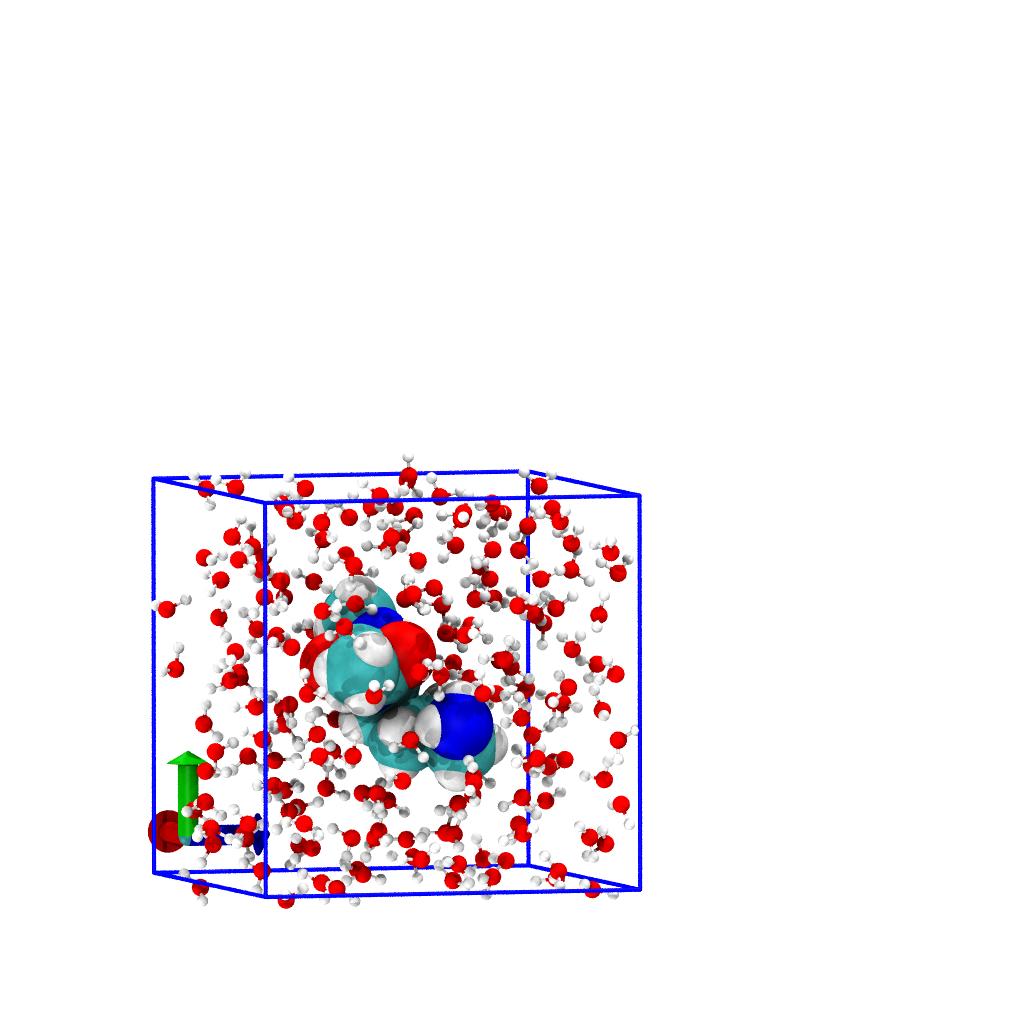
Then we also need to put all atoms inside the new unit cell newbox using AtomGroup.wrap()

smaller_system.wrap(compound="atoms", box=newbox, inplace=True)

With inplace=True we change the coordinates of all atoms in smaller_system directly.

The reduced system with its new smaller unit cell shown in blue. All atoms have been wrapped into the primary unitcell and bonds correctly extend "across" periodic boundaries.

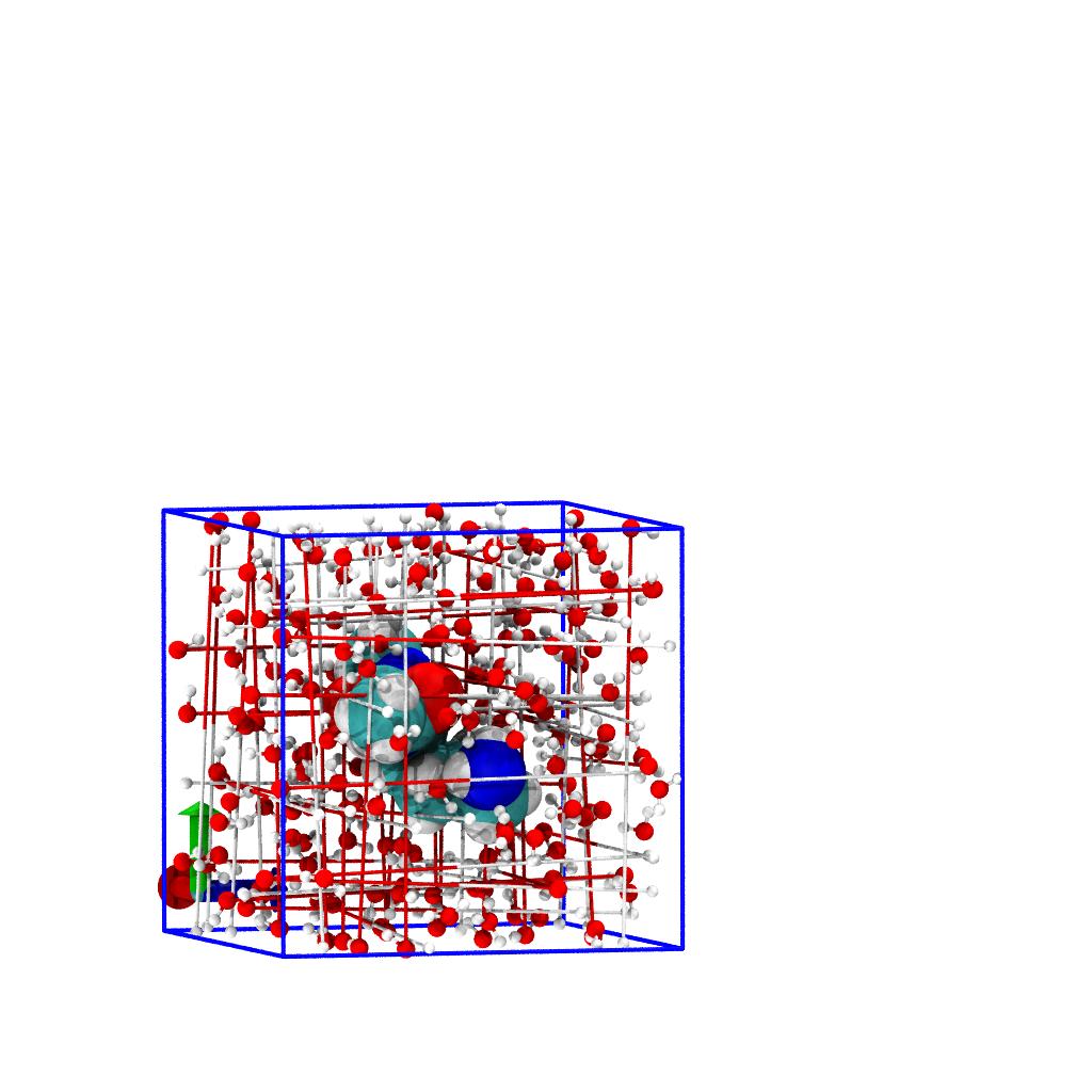
We now have cut out an orthorhombic subsystem and adjusted the unit cell information so that FHI-aims will be able to work with the system.

Output to geometry.in

We want to write the our reduced system to a FHI-aims geometry.in file (MDAnalysis supports reading and writing the FHI-aims file format). We take the atoms of our sub-system from the smaller_system.atoms attributes and use its write() method (which can determine the output format from the filename extension):

u.atoms.write("geometry.in")

We can also write a file in PDB format for visualization in tools that may not understand the FHI-aims format:

u.atoms.write("geometry.pdb")

(Ignore harmless warnings about attributes that are set to default values to satisfy the PDB standard.)

Suppressing warnings in Python

You can temporarily silence the warnings with the warnings filter:

import warnings
with warnings.catch_warnings():
    warnings.simplefilter("ignore", UserWarning)
    smaller_system.write("geometry.pdb")

Complete script

Save this script as extract_reduced_pbc.py:

# -*- coding: utf-8 -*-
import warnings
import numpy as np
import MDAnalysis as mda
from MDAnalysis import transformations

u = mda.Universe("./files/MD/NPT/md.tpr", "./files/MD/NPT/md.trr")
u.atoms.names = u.atoms.elements
water = u.atoms.select_atoms("resname SOL")
solute = u.atoms.select_atoms("resname ACE LYSN NME")
assert u.atoms == solute + water

workflow = [transformations.unwrap(u.atoms),
            transformations.center_in_box(solute, center='geometry'),
            transformations.wrap(water, compound='atoms')]
u.trajectory.add_transformations(*workflow)

u.trajectory[-1]

# bounding box of the peptide
bbox = solute.bbox()
A, B, C = bbox[1] - bbox[0]
print("unit cell:   a={uc[0]:7.4f} Å  b={uc[1]:7.4f} Å  c={uc[2]:7.4f} Å  ⍺={uc[3]}° β={uc[4]}° ɣ={uc[5]}° ".format(uc=u.dimensions))
print(f"solute bbox: A={A:7.4f} Å  B={B:7.4f} Å  C={C:7.4f} Å")

# additional distance in all directions
delta = 5
rmin = bbox[0] - delta
rmax = bbox[1] + delta

# select complete molecules with "byres" inside the extended box around
# the solute
water_box = water.select_atoms(f"byres prop x > {rmin[0]} and prop x < {rmax[0]} and "
                               f"prop y > {rmin[1]} and prop y < {rmax[1]} and "
                               f"prop z > {rmin[2]} and prop z < {rmax[2]}")
# combined system
smaller_system = solute + water_box

# new unit cell: A, B, C, alpha, beta, gamma
newbox = np.concatenate([rmax - rmin, [90, 90, 90]])

# Put all atoms inside the new unit cell
u.atoms.translate(-rmin)
smaller_system.wrap(compound="atoms", box=newbox, inplace=True)

smaller_system.dimensions = newbox

smaller_system.write("geometry.in")
with warnings.catch_warnings():
    # write PDB output without the needless warnings about defaults for the PDB file
    warnings.simplefilter("ignore", UserWarning)
    smaller_system.write("geometry.pdb")

Adjust the input files and the selection criteria and then run it with

python extract_reduced_pbc.py

Energy minimization for the reduced system

The resulting geometry.in is probably not yet suitable as input for FHI-aims due to steric clashes.

Finding clashes

We can find all interatomic distances in the small_system below a cutoff (say, 2 Å) with MDAnalysis using the fast MDAnalysis.lib.distances.self_capped_distance() function:

import numpy as np
from MDAnalysis.lib import distances

pairs, dist = distances.self_capped_distance(
                  smaller_system, max_cutoff=2, 
                  box=smaller_system.dimensions, return_distances=True)

The array dist contains the distance for each pair of atoms in the pair list pairs, taking the periodic boundaries into account via the box=smaller_system.dimensions argument.

A histogram of the distances shows us immediately that there are a number of contacts \(< 0.8\) Å (which is much closer than a typical bond length involving hydrogen).

Plotting the distance histogram

The distance histogram can be immediately obtained from dist with numpy/matplotlib:

import matplotlib.pyplot as plt
plt.hist(dist, bins=25)
plt.vlines(0.8, 0, 400, colors="black", linestyles="--")
plt.xlabel(r"interatomic distance $d$ (Å)")
plt.ylabel("counts")

Histogram of the interatomic distances in the reduced system. The vertical dashed line at 0.8 Å indicates that approximately all occurences less than 0.8 Å are indicative of clashes that were introduced by wrapping the water molecules into a smaller unit cell.

In this example, the number of atom pairs that are clashing are

>>> np.sum(dist < 0.8)
13

The explicit distances are

>>> dist[dist < 0.8]
>>> array([0.68607039, 0.76228015, 0.45474766, 0.73319411, 0.71172214,
           0.69234899, 0.41190428, 0.7202629 , 0.58936537, 0.49754758,
           0.51289614, 0.53577986, 0.66571993])

We can find the pairs with

>>> pairs[dist < 0.8]
>>> array([[340, 229],
           [424, 181],
           [423, 181],
           [182, 425],
           [203,  62],
           [587, 556],
           [585, 556],
           [585, 555],
           [590,  69],
           [590,  71],
           [491, 411],
           [491, 412],
           [411, 489]])

where each tuple consists of the atom indices of the two atoms. We can also directly index the AtomGroup smaller_system with these indices to get more information; here we just print to quickly convince ourselves that these are distances between different water molecules (indicated by different residue IDs ("resids")) and therefore these are almost certainly clashes that we introduced:

>>> clashes = [smaller_system[pair] for pair in pairs[dist < 0.8]]
>>> print(clashes[0])
>>> <AtomGroup [<Atom 1475: H of type HT of resname SOL, resid 484 and segid seg_1_SOL>, <Atom 815: H of type HT of resname SOL, resid 264 and segid seg_1_SOL>]>
>>> [clashgroup.resids for clashgroup in clashes]
>>> [array([484, 264]),
     array([678, 195]),
     array([678, 195]),
     array([195, 678]),
     array([224,  31]),
     array([948, 885]),
     array([948, 885]),
     array([948, 885]),
     array([955,  36]),
     array([955,  36]),
     array([757, 661]),
     array([757, 661]),
     array([661, 757])]

Removing clashes with energy minimization

One can take different approaches to reduce/remove the clashes. Here we use the classical force field approach again and do an energy minimization ("geometry optimization") with the GROMACS MD program.

Note

In order to do this part of the tutorial you need to have a working GROMACS installation as described in Running the classical MD simulations.

The main considerations are

• The unit cell is so small that the normal cut off distances for the neighbor list and non-bonded cutoffs are too large. We have to reduce them to values smaller than half the box size. Under normal circumstances we would not use such small values, especially as the force fields are parametrized with specific values for the VDW/LJ interactions. For the purpose of removing clashes, these are acceptable compromises.

• To better capture the physics of the small periodic system we use Ewald VDW (PME VDW) in GROMACS, which computes LJ in the periodic system without a cutoff. This is generally more expensive and the CHARMM force field was parameterize with LJ cutoffs so normally we would use cutoffs at the literature values. If PME LJ is not available then LJ with short cutoffs should also work as we are primarily concerned with close contacts.

• We will use two separate energy minimizations:

  1. First with no constraints on any bonds to allow all water molecules to easily rearrange. Water molecules were simulated with the rigid TIP3P water model which has all interatomic distances fixed with SETTLE constraints. By replacing constraints with bonds for this step, we give the molecules more freedom to relax clashes without running into numerical instabilities when constraints cannot be easily satisfied. We use a moderate convergence criterion (emtol) of maximum force of 1000 kJ/mol/nm = 1.036 eV/Å. We can use the excellent L-BFGS minimizer for this step.

  2. In the second step we enable constraints again to pull water molecules into shape. We use a simple and robust steepest descent minimizer but now use a fairly strict (for classical force fields) convergence criterion of 100 kJ/mol/nm = 0.104 eV/Å.

Directory set up

In the following we work in a directory EnergyMinimization. Create two separate work directories

mkdir EnergyMinimization && cd EnergyMinimization
mkdir topology energy_minimization

We use the geometry.pdb file that we wrote out previously. Copy it to the topology directory together with all topology files that were necessary for Running the classical MD simulations

• topol.top: topology file (overall system information)
• aceKnme.itp: included topology file (information for the lysine dipeptide)
• posre.itp: position restraints (not needed but referenced in topol.top)

Info

All input files are also downloadable from files/EnergyMinimization.

Update topology file

Edit the topol.top file to update the number of water ("SOL") molecules. Get the number with water.n_residues (in Python) or grep '^ATOM.*SOL.*O' geometry.pdb | wc -l (in the shell). Your molecules section should look like

[ molecules ]
; Compound        #mols
aceKnme           1
SOL               195

First energy minimization without constraints

We run an initial energy minimization with the L-BFGS minimizer and distable all constraints by using constraints = None and selecting water topology files for "flexible" water, i.e., where bonds are not constrained with SETTLE (-DFLEXIBLE). The important lines in the MDP file 01_emin_noconstraints.mdp are

define                  = -DFLEXIBLE
integrator              = l-bfgs
emtol                   = 1000.0
...
constraints             = None

As mentioned above, all cutoffs need to be shortened to less than half the box lengths so that the non-bonded section looks like

rlist                   = 0.5
vdwtype                 = PME
lj-pme-comb-rule        = Geometric
rvdw                    = 0.5
coulombtype             = pme
rcoulomb                = 0.5

MDP parameters

For further details on setting simulation parameters see Molecular dynamics parameters (.mdp options) in the GROMACS manual.

The MDP file for this minimization step can be downloaded from 01_emin_noconstraints.mdp.

We now generate the portable binary run input file for GROMACS with the gmx grompp command

gmx grompp -maxwarn 1  -f 01_emin_noconstraints.mdp  -c ../topology/geometry.pdb -p ../topology/topol.top -o 01_emin.tpr

where we use our geometry.pdb as input for the starting coordinates and 01_emin_noconstraints.mdp sets the run parameters. We have to use -maxwarn 1 to ignore one harmless warning about mismatching atom names (because we renamed atoms to elements for FHI-aims).

We can then run the minimization itself with gmx mdrun

gmx mdrun -nt 1 -deffnm 01_emin -s 01_emin.tpr

The L-BFGS minimizer only runs in serial so we set the number of threads to 1 (-nt 1) for gmx mdrun. The run should produce output files 01_emin.{gro,tpr,log,edr} within seconds. The log file should indicate that the minimization converged:

Low-Memory BFGS Minimizer converged to Fmax < 1000 in 43 steps
Potential Energy  = -6.5631802e+03
Maximum force     =  8.5441931e+02 on atom 5
Norm of force     =  2.6728458e+02

Second energy minimization with constraints

In the second energy minimization step we enable constraints for bonds involving hydrogens again (which are solved with SETTLE for water and LINCS for everything else) and use a tighter convergence criterion. The run input MDP file 02_emin_constraints.mdp contains

define                  = 
integrator              = steep
emtol                   = 100.0
...
constraints             = h-bonds
constraint_algorithm    = LINCS

Generating the TPR file and running the minimization follows the same protocol as before,

gmx grompp -maxwarn 1  -f 02_emin_constraints.mdp -c 01_emin.gro  -p ../topology/topol.top -o 02_emin.tpr
gmx mdrun -nt 4 -deffnm 02_emin -s 02_emin.tpr

Note that the starting coordinates are read from the output of the previous energy minimization, 01_emin.gro. The minimization can be run in parallel and 4 threads (-nt 4) should make this task finish in a couple of seconds. The output should show convergence, e.g.,

Steepest Descents converged to Fmax < 100 in 1524 steps
Potential Energy  = -9.8530654e+03
Maximum force     =  9.2342125e+01 on atom 5
Norm of force     =  1.4365285e+01

The final energy minimized coordinates are in the 02_emin.gro file.

Check energy minimized geometry for clashes

We analyze the interatomic distances for clashes (\(d < 0.8\) Å) as before, but we now load the final energy minimized coordinates in the 02_emin.gro file. Load the final coordinates into a MDAnalysis Universe and calculate the distances:

em = mda.Universe("EnergyMinimization/energy_minimization/02_emin.gro")
pairs, dist = distances.self_capped_distance(em.atoms, max_cutoff=2, 
                                             box=em.dimensions, return_distances=True)

How many distances are below our clash distance?

>>> np.sum(dist < 0.8)
0

Zero! This indicates success, we removed all clashes.

Convert GROMACS output to AIMS geometry.in

We use MDAnalysis to convert the coordinates in 02_emin.gro to a geometry.in file as before:

import MDAnalysis as mda

TPR = "02_emin.tpr"
GRO = "02_emin.gro"

AIMSIN = "geometry.in"
PDB = "geometry.pdb"

u = mda.Universe(TPR, GRO)
u.atoms.names = u.atoms.elements

u.atoms.write(AIMSIN)
u.atoms.write(PDB, remarks="energy minimized with GROMACS")

The resulting geometry.in file should now be suitable for calculations in AIMS. In particular, the density SCF iterations should converge.