Introduction

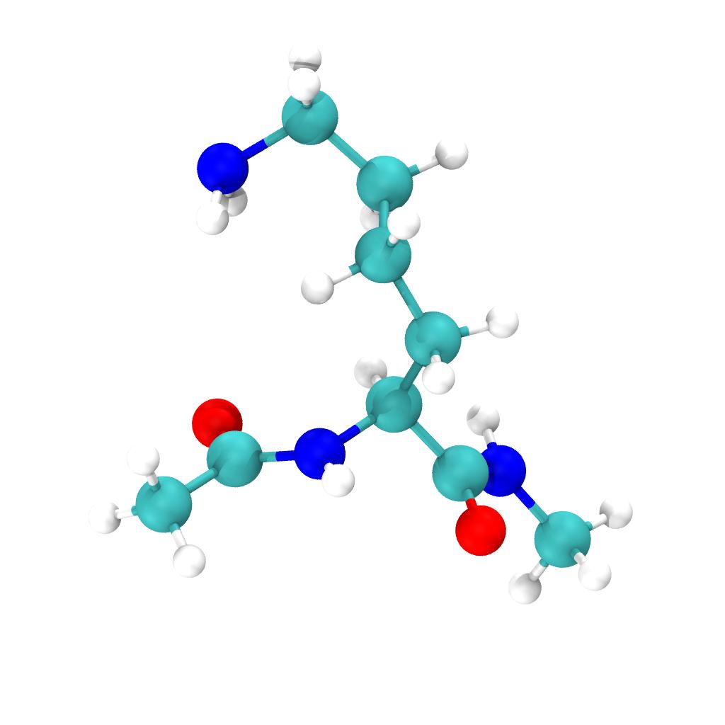
For this tutorial we look at a capped lysine amino acid solvated in water that has been simulated with classical molecular dynamics (MD). We show how to extract either the whole system or a subsystem with MDAnalysis for simulation in FHI-aims.

We simulate the lysine in its deprotonated (neutral) form and we acetylated the N-terminus and N-methylated the C-terminus of the amino acid to remove any zwitterions.

Capped lysine amino acid with deprotonated amino group (NH₂-) and neutral N-terminus (acetylated) and C-terminus (N-methylated).

Objectives

We want to

1. solvate the amino acid in water and simulate it with classical molecular dynamics (MD) to obtain reasonably realistic conformations;
2. write out frames of the simulations (potentially only part of the classically simulated system) as input for ab-initio MD with FHI-aims.

In this tutorial we will show how we can use MDAnalysis to convert the whole classical MD system or subsystems into a geometry.in file suitable for FHI-aims.

The classical MD is performed under periodic boundary conditions to minimize boundary artifacts, with long range electrostatics with Particle-Mesh Ewald for the Coulomb interactions and truncated Lennard-Jones (van der Waals) interactions. The cutoff of the LJ interactions of 1.2 nm (for the CHARMM36 force field) necessitates a simulation box that may already be bigger than what we want to simulate at the ab-initio level so we are looking for a way to extract a smaller subsystem,

The primary consideration is if we want to perform simulations in FHI-aims with periodic boundary conditions (using the k_grid keyword) or non periodic simulations (no k_grid, possibly with use_hartree_non_periodic_ewald).

Pre-requisites

In the following we assume that you installed MDAnalysis (typically in a conda environment). All classical MD simulations have been performed and the necessary files are available in the files/MD/NPT folder. (Any other folders under MD are only needed if you want to run the classical MD yourself.)

Input files

Download or copy the files from files/MD/NPT. In particular you will need

• md.tpr: binary run input file for GROMACS that contains atom type and bond information (as well as all information to run the simulation, see NPT MD (production).
• md.trr: full precision GROMACS MD trajectory with positions and velocities saved every 100 ps for a 1 ns trajectory (NPT ensemble at T=300 K and P=1 bar).

Optional files (not needed for the tutorial itself):

• md.gro: final conformation of the trajectory at 1 ns in GRO format; useful for visualization with tools that cannot read the TPR file.
• md.mdp: GROMACS run parameter file; not needed for this tutorial unless you want to know exactly how the classical MD simulation were performed or if you want to run them yourself.

Learning MDAnalysis

We recommend that you learn the basics of MDAnalysis by looking at the Quick Start Guide.

Additional help is available in the User Guide.

If you have questions, participate in the MDAnalysis Community via Discord or mailing lists.

Optional: Run the classical MD simulations yourself

If you want to run the MD simulations yourself, then the necessary input files and steps are described in the optional Running the classical MD simulations.